We made experiment queries 4x faster using precomputation

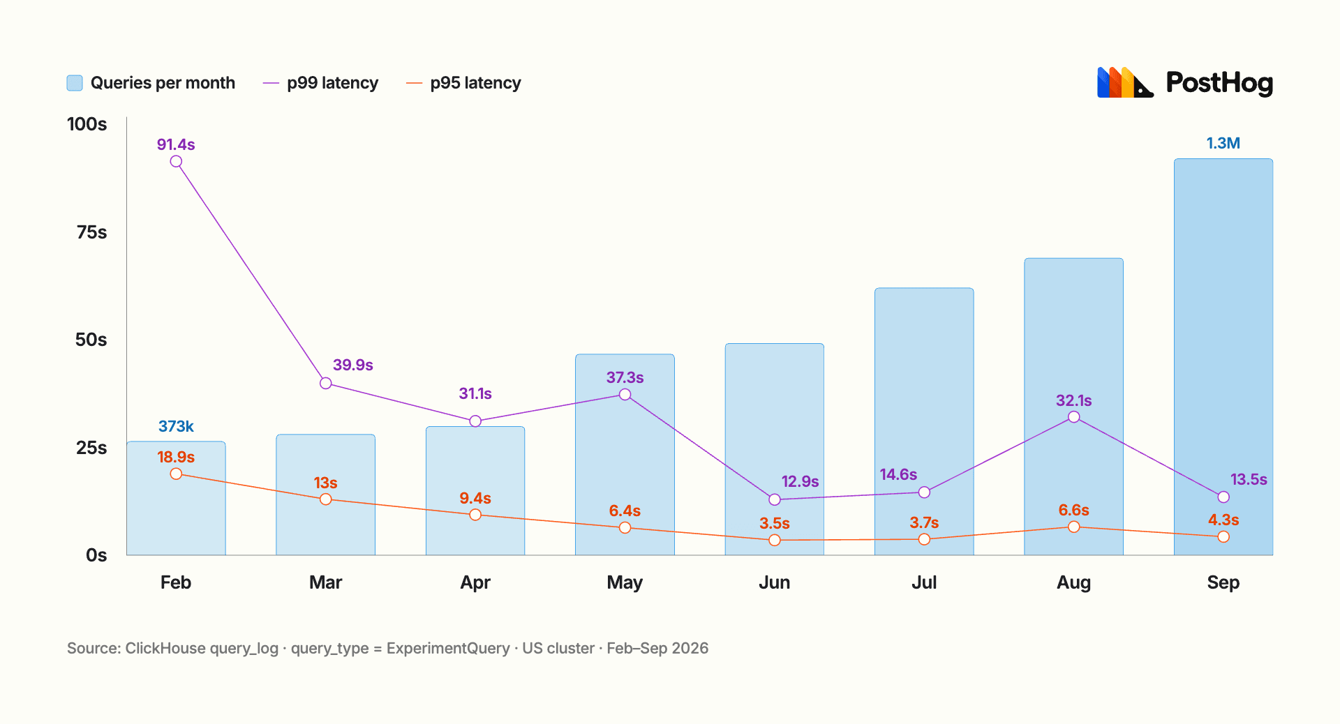
In February, the p95 latency of our experiment queries was 19 seconds, and the slowest 1% took over a minute and a half. Queries regularly died because they timed out, ran out of memory, or scanned more data than our cluster allowed.

By September, p95 was down to 4 seconds and those failures were 14 times rarer, while monthly query volume more than tripled. This post is about what we did to make this happen.

Some context about Experiments in PostHog

PostHog Experiments first shipped in December 2021 as a very minimal tool. Built on top of our Feature Flags, it was initially just a simple wrapper around Product Analytics – a single funnel query with some statistical calculations on top.

Over time, it evolved into a mature experimentation product. Today, we support many different metric types and aggregations, Data Warehouse sources, Bayesian and frequentist statistics, CUPED for variance reduction, winsorization for handling outliers, and holdout groups for measuring long-term effects of experimentation. If you need a mature experimentation tool, it's all here under one roof in PostHog.

As our product grew, our customers did too. From a handful of small customers, we've grown to serve some of the fastest-growing startups in the world. Some of them send hundreds of millions of events per day, with individual metric queries scanning terabytes of data.

By early this year, our system was choking on the load, and many of our largest customers were struggling to load their metrics. Fixing this was a large undertaking, and we attacked it from multiple angles.

1. Build a precomputation system

Author Robbie CoomberRobbie Coomber

Our first step was to spin off a query performance team with the aim of improving query performance across the entire PostHog platform. We quickly built an MVP of query precomputation: a library that different teams could use to precompute their queries.

There are different kinds of queries, but the kind this applies to best is a timeseries query – a series of time buckets over some range of time, which is exactly what experiments use.

Here's how precomputation works.

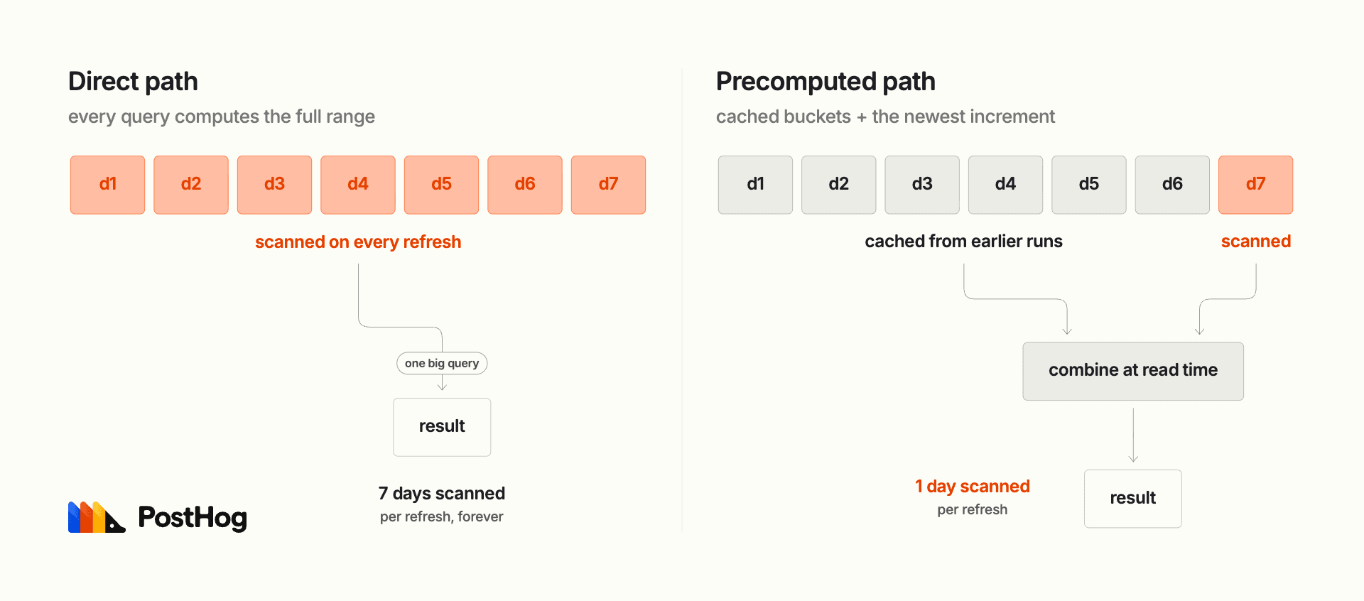
Suppose you start your experiment. It's day 1 and you load your first results. Instead of throwing away the data that query computed, we persist it in the database. Then on day 2, you ask for results for the entire time range (now 2 days). Instead of querying day 1 + day 2, we retrieve the stored data for day 1, query only day 2, and combine the two.

This avoids double work: each query only scans the latest increment. Repeat this every day: by day 7, we read six cached buckets and scan only one.

In practice, this is more involved than the example above. Because in analytics we have events arriving late (perhaps from a mobile app that was offline for some time), we need to drop cached data after some time and re-query, to make sure our results are up to date.

The refresh schedule backs off with age: the older the bucket, the less likely it is that late events will still arrive for it, so it can stay cached for longer. Roughly, it works like this:

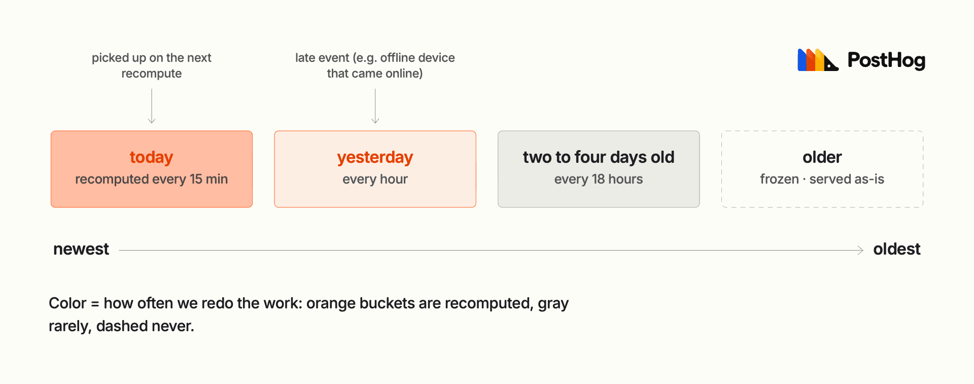
There's a tradeoff here: events that arrive after their bucket is frozen are missing until the data expires and is rebuilt. For experiments this is acceptable. You aren't checking results every single minute; you let the experiment run for a couple of days or weeks and then conclude, so tiny inaccuracies are acceptable.

With some production testing, we found a good balance between not doing too much work and keeping results accurate and consistent. We have production checks that monitor consistency here – more on that below.

2. Integrate precomputation into Experiments

Author Juraj MajerikJuraj Majerik

Experiments was the first product to use the precomputation library, and we tested and improved it by operating it in production.

Integrating the library was itself a big task. We have four different metric types, each with different aggregations. Then there are optional breakdowns, and experiments that aggregate by users or by groups.

This creates many possible combinations, and precomputation needs to work for each of them. We store everything in a single table, but that single table needs to support all the different data shapes.

For each of the four metric types in the precomputation path, we had to write new queries. These queries differ from the default "direct" path shown in the diagram above.

The direct path does everything in a single query: it scans the events, filters them, and computes the final result. The precompute path splits this in two: a write query stores the matching events in the cache, and a read query aggregates them later.

The write query cannot compute final results, because data from many separate day buckets has to be combined at read time. So the direct and precomputed paths express the same logic in different ways, and they have to match perfectly.

We did this progressively and incrementally. There are many moving parts, and part of learning how it all fits together is simply building it, running it in production, and testing with a couple of select customers first. We still ran into problems we didn't foresee. While we do have a comprehensive integration test suite, it didn't catch all the issues.

The biggest issue we ran into: a pilot customer had a metric return three different results in quick succession – in one case, the results were 35.2%, 41.6%, and 56.9%, just seconds apart. They had this correctness problem for several days, and we only found out after they complained.

The issue was with ClickHouse, which we use as the cache. ClickHouse is a distributed database: data lives spread across several nodes. When you insert, one node accepts the rows and then forwards them to the nodes that store them – and by default, that forwarding happens asynchronously.

So, we wrote the data, got an acknowledgment back, and marked the cache as ready, while the rows were still on their way to the other nodes. A read that followed immediately saw only part of the data, so it returned a lower number. As the remaining rows arrived, each following read saw more of the data, which is why the number kept changing.

The fix in this case was simple: make the insert synchronous, so the write only returns once the nodes storing the data confirm they have it. This is a configuration change, not a code change. But it was a wake-up call. We had missed the issue because our integration tests run on a single ClickHouse instance, where these problems cannot appear. We knew we couldn't rely on tests alone going forward.

We caught other issues, too. Cached buckets were aligned to calendar days in UTC, so an experiment started mid-day pulled in events from before its start, and some users ended up misclassified.

In another case, our cache-filling queries didn't apply the same settings as regular queries, so a filter involving missing property values silently dropped rows and left the cache nearly empty. These were less serious, but they were still correctness issues in edge cases.

To solve this uncertainty for good, we built a comprehensive canary testing suite running on production data.

Each night, a background job picks a random set of metrics and runs each of them in both modes: the direct-scan mode, which reads the entire time range, and the precomputed mode, which reads the cached data. Then we compare the results.

If they diverge beyond a small tolerance, we get an alert. The canary also caught the issue of late-arriving events and helped us tune the cache invalidation times.

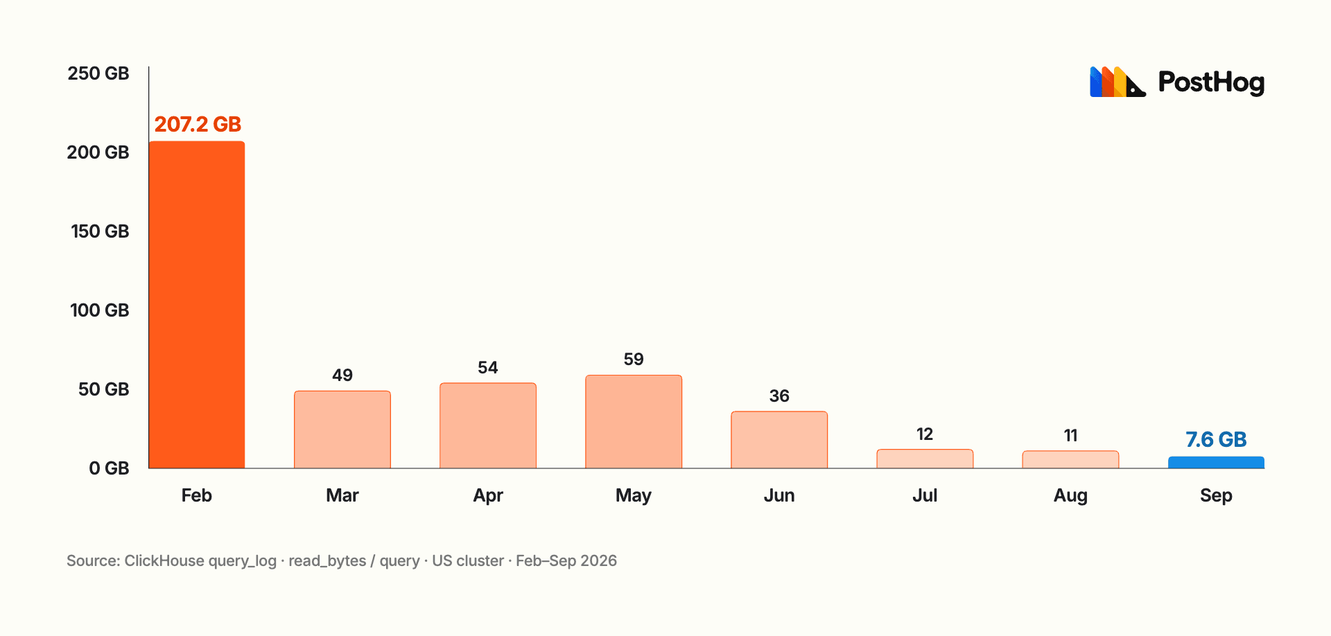
The payoff of all this work is visible in how much data a query needs to touch:

3. Optimize the SQL

Author Anders Asheim HennumAnders Asheim Hennum

Experiment queries need to work out who was exposed to a variant and what those people did afterward. Both sets of data come from the events table, and combining them per user adds to the cost of reading billions of rows.

Our funnel query used to scan the table twice, once for exposures and once for metric events. We rewrote it to collect both in a single scan, keeping the timestamps needed to evaluate the funnel in the right order. As a result, an example production query we tested went from 16 seconds to 8 seconds.

-- Before: two scans of the events table
SELECT ... FROM events WHERE event = '$experiment_exposure'
SELECT ... FROM events WHERE event IN ('purchase', 'signup')

-- After: one scan, with exposures and metric events separated during aggregation
SELECT ... FROM events WHERE event = '$experiment_exposure' OR event IN ('purchase', 'signup')

Other metric queries had a different problem: they ran out of memory while joining the two sets of data. The join kept one side entirely in memory, which became too expensive for large queries. We switched to an algorithm that processes the data in smaller batches and keeps the rest on disk. That adds disk reads and writes, so it can be slower, but it lets a query finish when the previous version would have failed.

We also found an expensive read that the metric calculation didn't need. Clicking a funnel step shows session recordings of users who reached it, and finding those recordings required a session ID stored inside each event's properties. That meant reading the largest column in the events table for every scanned row, even if nobody opened a recording. We moved the lookup into a separate query that runs only when someone uses the feature.

4. Use a dedicated exposure event

Author Anders Asheim HennumAnders Asheim Hennum

For a long time, we used an event called $feature_flag_called to track experiment exposure. This event also records evaluations of flags unrelated to experiments, so most of that traffic wasn't useful to an experiment query.

Reusing the event made sense when Experiments was small, but our large customers were now accumulating tens of millions of flag events a month. Every query had to find the relevant exposures among all that data.

We added a dedicated event, $experiment_exposure, which records assignments to flag variants. We create it during ingestion from the flag events customers already send, so the change needed no SDK updates.

These exposure events are roughly a tenth of the volume of flag events, giving experiment queries a much smaller set of data to read.

5. Move recalculation to Temporal

Author Rodrigo IloroRodrigo Iloro

Until recently, when you opened an experiment with 30 metrics, your browser issued API calls for all 30 results at once. This is a problem, as we only allow a team 10 concurrent queries – a limitation designed to protect our ClickHouse cluster.

The remaining 20 would keep retrying until slots freed up, but that waiting counted toward their timeouts. Refreshing the page could then submit the same 30 queries again while the first batch was still running.

We moved recalculation to Temporal, a system for running long tasks reliably. It records the progress of each recalculation, so after a crash or restart we can continue with the unfinished work.

When you refresh the page now, you reconnect to the calculation that's already running, and failed metrics can retry while the others finish. We can also see what happened during a run, which was much harder when the browser was coordinating the requests.

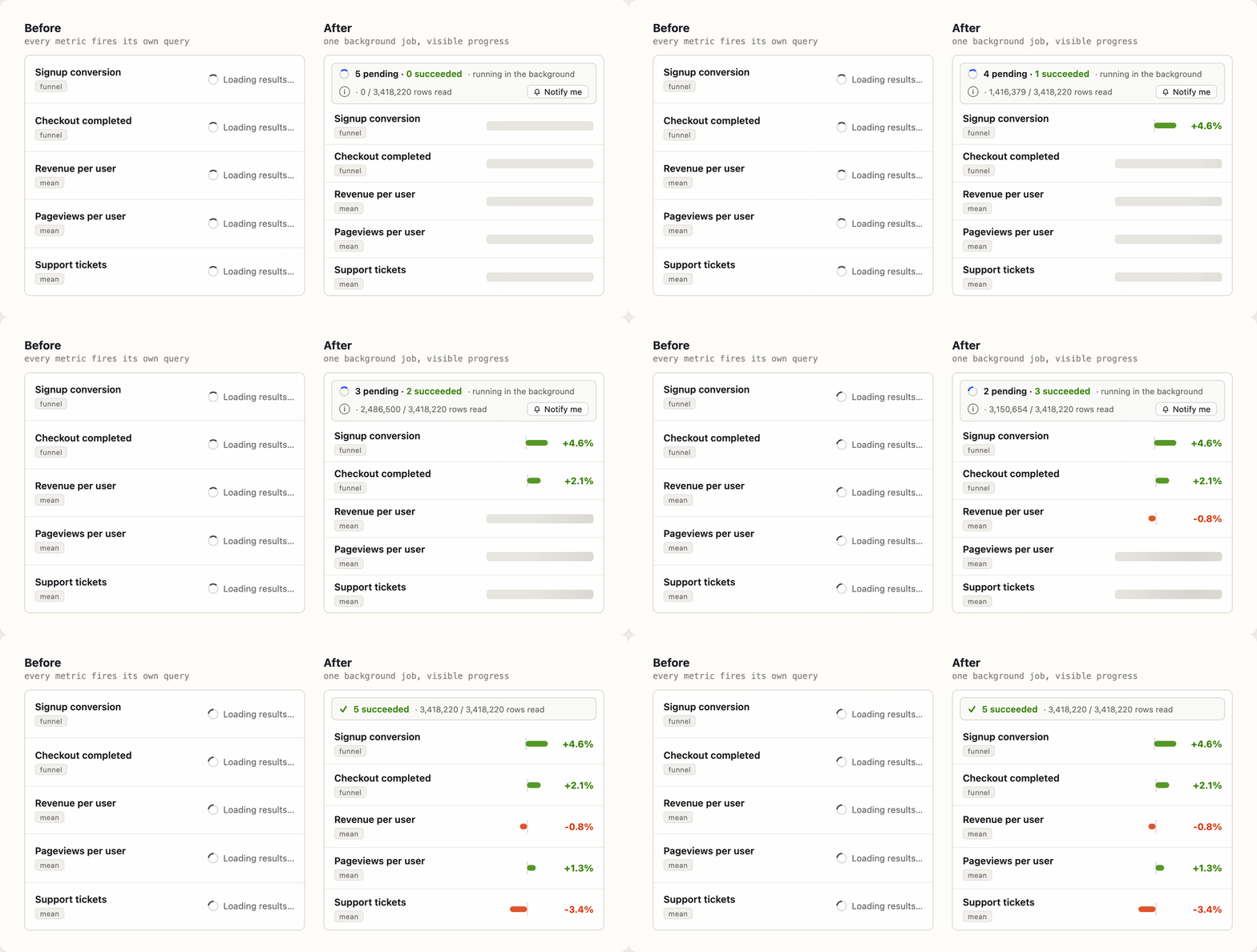
A lesson we learned here is that query performance is also about perception – it really matters how you present waiting to the user. When issuing requests from the browser, we would show a bunch of spinners. But spinners create an expectation of immediacy, with very little transparency into what's going on. If a query takes a minute to load, this makes for a poor user experience.

Here's what we do now: we show a banner with a clear overview of how many queries are pending, how many are executing, and which have already completed. This is much better, as the user now understands that this is not a simple query, but an orchestrated background job, potentially heavy (indicated by rows read), with some metrics waiting in a queue.

Some queries will still take a long time. This is unavoidable. Sometimes you cannot use precomputed data at all: if you add a completely new metric, or change the experiment in a way that affects the calculation, there is no cached data to reuse yet.

A query for a large customer might simply take a long time, but it really matters how you present this background process to the user and what expectations it creates.

How AI helps us run this

A system like this generates a constant stream of small questions:

• Why did this query slow down?
• Why did the canary flag this metric?
• Why is this team suddenly reading ten times more data than last week?

The answers are almost always somewhere in Grafana, or in the ClickHouse query log, but digging them out by hand is slow.

So we connected AI agents to these tools. Now we describe the problem in a prompt and get an investigation back minutes later. When the nightly canary flags a divergence, an agent pulls the logs and reconstructs which experiment and metric went wrong, and how.

When we planned the precomputation work, an agent mapped out every path a query can take through our system and how expensive each one is. We integrated the busiest paths first and the rarest ones last – some of them we still haven't needed to do. This is the same instinct behind pointing an agent at our query engine and letting it run overnight.

The agent doesn't fix anything for us. What it changes is the feedback loop: the time between "something looks off" and "we know why" went from hours to minutes. The charts in this post came out of one of these sessions.

What we learned

We avoided precomputation for a long time, and that was deliberate. We had worked on query performance before, but incrementally, mostly through SQL optimization.

As a small team competing against companies with hundreds of engineers, it was convenient to have just one simple, direct path that always calculates the entire time range. Caching is notoriously hard, and it made sense to keep our mental model simple for as long as possible.

Only when our customers started clearly struggling did we accept that we couldn't wait any longer. We also learned that an impressive integration test suite is not enough for a system like this. If something can break in production in ways your tests don't cover, it eventually will.

The added complexity may seem daunting, but we're in a much more stable place now. You can absolutely run a reliable, performant, and relatively complex system with a small team like ours.